Excel Lesson Plan - Expense Budget with Chart

Assignment: Students create a clothing expense spreadsheet budget with chart. Students use a shopping list to buy some clothes and tally their expenses. Students create a chart illustrating their clothing purchases and expenses.

Download: excel-clothing-expenses-with-chart-finished-example.xlsx

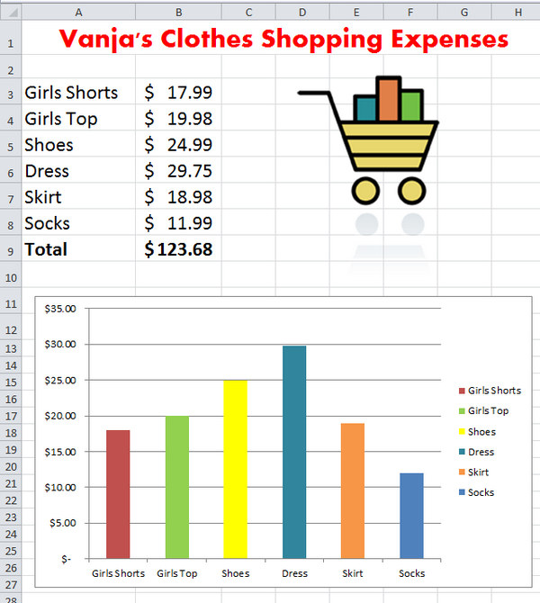
Excel Clothing Expense Budget & Chart - Finished Example

Download: excel-clothes-shopping-price-list.pdf

Clothes Shopping Price List:

Students choose items from this list for their spreadsheet entries.

Download: student-instructions-clothes-shopping-expenses.docx

Student Instructions

Excel Mini-Course in 4 Minutes:

Quickly learn the essentials you need for this lesson with these short, focused video tutorials. Watch all the videos to see how to create a budget and chart from start to finish or just watch the ones you need.

Students Learn and Practice
the Following Basic Spreadsheet Skills:

• Creating and formatting a spreadsheet title using "merge and center"
• Entering data in columns and rows
• Using the simple formula "Autosum" to automatically calculate total expenses
• Formatting numbers as currency and adding $ signs.
• Creating a chart using the expense data entered.
• Using different colors for chart segments to improve visual presentation
• Creating, sizing, and positioning the chart to fit on a single page with the data
• Searching, inserting, sizing, and positioning clipart or pictures
• Using print preview and printing

Download: rubric-for-spreadsheet-with-chart.pdf

Excel Spreadsheet Rubric for Grading Assignments