iWork Numbers - Make a 3D Bar Chart
|
|
Students Create and Format a 3D Bar Chart in iWork Numbers
These instructions are for iWorks Numbers '08, but the concepts and actions are similar for other versions. I have taught this level of spreadsheet and chart creation with 2nd graders and up. Your mileage may vary. Be sure to have students use "Show Print View" before printing to make sure the chart fits onto a single page to avoid wasting paper and ink.
This lesson builds on the first iWork Numbers First Chart by adding the following requirements:
Merge Cells for the table title. "Sean's Ice Cream Chart"
Apply formatting to the title such as font size, color, and style.
Enhance the 3D chart by using the Chart Inspector and labeling the chart title.
iWorks Numbers Tutorial
Use this mini iWorks Numbers tutorial to guide your students in entering the data and creating the chart.
1) Enter the title of the table in cell B1. In this example: Sean's Ice Cream Chart
2) Click in cell B1 and drag the selection to F1. On the Menu bar, go to Table > merge cells.
3) Change the font color, size and style of Sean's Ice Cream Chart text.
4) Enter the ice cream data into column A cells. Change the font color, size and style.
5) Enter the ice cream quantities into the column B cells. Change the font size.
6) Select (highlight) the ice cream and number data in columns A and B.
7) Click the Charts button on the menu bar and select the 3D bar chart.
8) The Chart Inspector displays options to adjust the chart. Change the chart colors here.
9) Double click the chart title and change it, in this example: Sean's Ice Party Ice Cream
10) Go to File > Show Print View to check how the chart will look before printing.
11) Drag the corners of the table as necessary until it fits into a single page in "Show Print View".
12) Print.
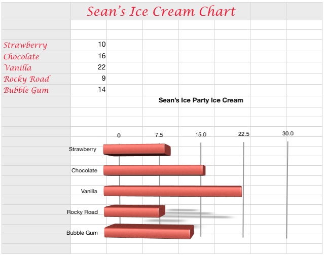
Finished iWork Numbers 3D Bar Chart Example:
